EpiStack — a Bayesian knowledge graph for contested empirical questions

Simon Skade · FLF Epistemic Stack competition

0 — Executive summary

I built a 10-step pipeline (a Claude Code skill, python scripts and a deterministic runner) that turns one contested empirical question into a typed, navigable Obsidian knowledge graph whose Bayesian answer recomputes from the notes.

Why this shape (§1): contested questions rarely lack evidence; what they lack is a way to navigate it. Counting who says what, weighted by prestige, then manufactures false confidence, because correlated sources get treated as independent voices. So the pipeline builds its own technical model bottom-up from low-level observations.

How to read the graph. Each node is one markdown file with typed YAML frontmatter plus prose, and each edge is a frontmatter wikilink, so the analysis directory is a directed typed graph. The answer is a report computed over the graph, never cached in it. No posterior, prior or likelihood sits in frontmatter, because cached numbers go stale silently.

Node types:

Type	Code	What it is
source	S	Primary paper or dataset
data-basis	D	Shared dataset, actor or instrument; observations sharing one are correlated
observation	O	Empirical finding
hypothesis	H	Candidate answer
hypothesis-cluster	HC	Mutually-exclusive answers to a sub-question, residual last
argument	A	Inference carrying no information of its own
evidence-link	E	Obs→cluster edge, minted only where it discriminates
correlation-group	CG	Joint likelihood for edges sharing a data basis

Four stages:

1. Ingest
   1. Find useful sources (steps 1 and 2, including data-reliability and provenance)
   2. Ingest into the knowledge base (3, extraction into observations)
2. Structure
   1. Hypotheses, clustered (4)
   2. Graph edges, i.e. discriminating evidence links (5)
3. Assess
   1. Argument validity (6)
   2. Bayesian analysis (7 and 8)
      1. Priors (7)
      2. Likelihoods (8)
   3. Additional abstract considerations, cluster review (9)
4. Assemble the final report (10)

Key features

The delta over off-the-shelf deep research or a single-prompt Claude Code run, most important first:

1. Correlated evidence is aggregated correctly. Observations resting on the same data-basis get one joint likelihood, not one factor each. Black-holes case: the folk “Earth and the Moon are still here” reassurance and the Giddings–Mangano stable-black-hole exclusion both resolve onto D-1 — High-energy cosmic-ray flux spectrum; a source-counter sees two independent reassurances, this pipeline one witness. D-1’s known_biases names their shared failure mode, fixed-target cosmic-ray kinematics mapped onto a collider’s near-symmetric kinematics. If that mapping is wrong, everything on D-1 fails together.
2. Source-trust is separated from claim-truth, so prestige cannot launder in. trust_score prices data-reliability from source features only; validity and truth are judged author-blind and must stay derivable with author and venue stripped.
3. Every number is an overridable named variable, its reason in the comment beside it. A skeptic re-prices any assumption and re-runs the whole model: --set BLOCK:var=value.
4. Uncertainty stays live. Every non-exhaustive cluster carries a residual member (“the answer is something not listed here”) with its own argued weight, never 1 − sum(others).

Provenance

Every file in each analysis folder is generated autonomously from initial_prompt.md by the single per-case command in §7, no hand-editing; retired nodes and agent notes are kept, so discards are auditable. Worked analyses: black-holes · eggs · covid.

Stated plainly: the pipeline is implemented end to end, the runner passes a self-check, and all three cases have run the whole way through step 10 as low-N shakedown runs. The §5.1 posteriors are real and recompute from the notes, but are small-N draws from much larger scored pools — a demonstration of the method, not settled answers.

§7 turns the black-holes run into a three-command demo, including a re-run that distrusts the single paper most of its likelihoods route through and watches the posterior move. Start there if you have a terminal.

---

1 — Underlying principles

A contested question rarely suffers from too little evidence. It suffers from evidence nobody can navigate. The usual shortcut (count who says what, weight by prestige) manufactures false confidence: correlated sources count as independent voices, and prestige and motivated framing launder in as truth. So rather than summarizing the debate, I modelled the question bottom-up from low-level observations, letting its framings earn their place or not. The graph is the artifact; the answer is a report computed over it.

1. Bottom-up carving. Hypothesis clusters come from what papers state and what observations can pull apart: step 4b forbids importing a tidy taxonomy of the debate, and step 4a’s merge test is “does any curated observation in scope come out differently under these two?” Why: top-down carving inherits the debate’s framing and its rhetorical seams. Where the evidence discriminates is a fact about the corpus, not the argument, so it must be discovered.

2. Numbers-as-variables. Every estimate is a named python variable with its reason commented beside it, in runnable blocks in the notes; steps 7 and 8 require reasoning sketched first, values filled last. Three payoffs. Legibility: a reader disagrees with the one step I got wrong, not an opaque aggregate. Skeptic-override: --set BLOCK:var=value re-runs the whole model with one assumption re-priced. Scaling: a stronger model re-estimates one variable in place without touching surrounding structure.

3. Trust ≠ truth. trust_score prices data-reliability from source features only (design, statistics, power, preregistration, independent replication, venue and citations only as a floor), and step 2 makes it prestige’s only sanctioned channel. Claim-truth (steps 7–8) and argument-validity (step 6) are judged independently. Otherwise reputation counts twice: as reliability, then again as plausibility. Enforcement: the verdict must stay derivable with author and venue stripped. Surprisingness is banned from trust too; it belongs to the prior.

4. Correlated evidence counted once. Observations resting on the same data-basis node get ONE joint likelihood on a correlation-group node, stating P(all of them | H). Why: independent-counting of correlated evidence is the standard way Bayesian aggregation manufactures false confidence, and what most separates this from a source-tally. Live instance in §4: two apparently independent black-hole safety arguments on one cosmic-ray dataset.

5. Explicit out-of-model residual. Every non-exhaustive cluster carries a residual member (“something not listed here”) with its own argued weight and real likelihood, never 1 − sum(others). Why: a complement is a rescaling artifact rather than an estimate, and it hides both failure modes. Too small and no evidence can lift it; too large and it soaks up every posterior. An argued weight keeps unmodelled explanations visibly competing.

Scalability

No hand-designed human bottleneck sits anywhere. One command per case produces every file, and the optional human-review mode is not load-bearing. The design improves with stronger models and more compute: better models re-estimate variables in place or extract more carefully, with no schema change; more compute buys more sources, deeper extraction, optional cross-model ensembling. Models are assigned per step by the orchestrator, on top of whatever session model the run was launched with (--model fable in §7). Judgment-heavy children (step 1’s planner and consolidator, both step-2 sub-steps) run on opus, searchers on sonnet, and everything else inherits the session model.

---

2 — The pipeline in detail

Ten steps, one orchestrator spawning every child. Each step fans out over disjoint slices and only adds to the previous step’s graph. No human checkpoints.

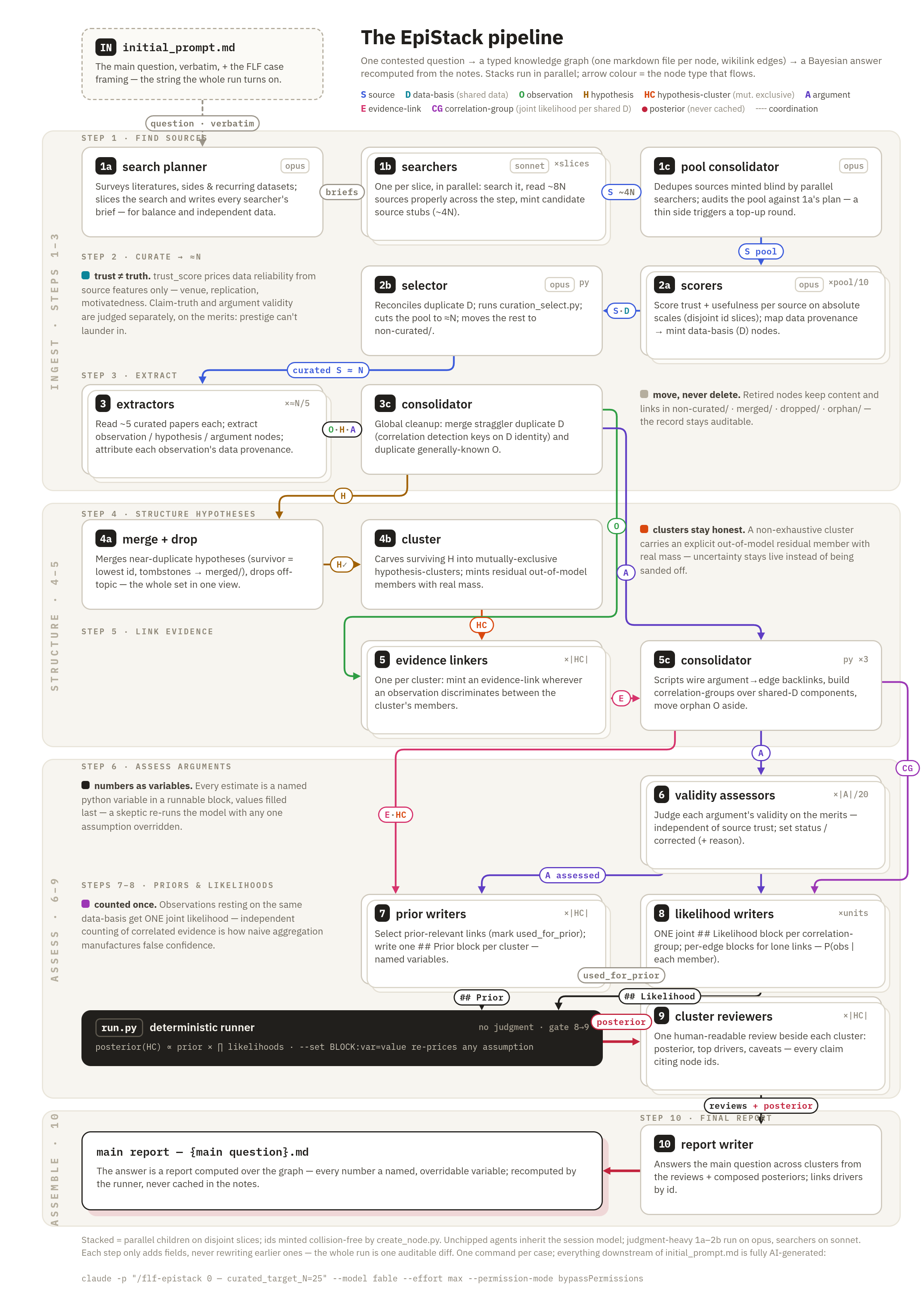
Arrow colour and label name the node type flowing along it; stacked boxes are parallel children on disjoint slices. The chips on the right of a box give its model and its fan-out.

The streams

Beyond §0’s node types: D turns “these two findings share a basis” into node identity rather than a free-text match. A CG is a connected component of edges sharing a D.

The steps

1. 1a planner. One child-prompt per slice. Judgment: how to slice, with independent data per slice and every side represented.
2. 1b searchers. S notes (~4N written, ~8N read) plus an orientation note. Judgment: the primary artifact, not the review citing it.
3. 1c consolidator. Deduped pool, audited against 1a’s plan; a thin side or data axis triggers a top-up round.
4. 2a scorers. Mint trust_score/usefulness, D nodes and each source’s data_basis. Judgment: would this survive a clean replication.
5. 2b selector. Duplicate Ds merged, ~N flagged curated. Judgment: the cut, trading a ranking point for data_basis independence.
6. 3 extractors. ~5 papers each, read in isolation; each O/H/A rests on exactly one source. Judgment: the observation/hypothesis line, i.e. what a rival team on the same data must grant.
7. 3 consolidator. Merges duplicate Ds and near-duplicate generally_known observations. Judgment: is this the same fact; paper-derived observations are never merged.
8. 4a merge/drop. Near-duplicate H merged, off-topic dropped. Judgment: discriminability; merge only where no in-scope observation would differ.
9. 4b cluster. Mints HC, residual members, backlinks. Judgment: the carving (one sub-question, exclusive answers, comparable grain).
10. 5 linkers. Mint an E only where a cluster’s members predict the observation materially differently. Judgment: diagnosticity; no numbers.
11. 5 consolidator. Attaches arguments via affects_observations, mints the CG nodes, orphans unlinked observations. No judgment: two scripts plus a sweep.
12. 6 argument batches. ≤20 each; approved/corrected/rejected plus checked/trusted out. Judgment: does the inference hold given its premises. Validity, not strength or truth.
13. 7 prior children. A ## Prior python block per cluster, used_for_prior: true on each edge spent. Judgment: the partition into base-rate and discriminating evidence.
14. 8 likelihood children. ## Likelihood blocks, one per CG or per ≤3 lone edges. Judgment: P(obs given member) as ratios, t capped by trust.
15. 9 cluster reviews. One per cluster, read-only. Judgment: what the model cannot express.
16. 10 report writer. One answer out. Judgment: weighing sub-answers given in different currencies. Written, not computed.

Two structural facts

1. The run is an auditable diff. Steps only add fields, never rewrite them; nothing is deleted. Retired nodes move to non-curated/, merged/, dropped/, orphan/, links and content intact, reason recorded.
2. The conclusion lives in the notes. runner/run.py executes the step-7 ## Prior and step-8 ## Likelihood python blocks to compose each cluster’s posterior; no derived number is cached in frontmatter. It gates between steps 8 and 9, so no review is written on a broken model.

---

3 — Why this ontology

Each node type exists because some later step judges it alone. An observation’s data-reliability, a hypothesis’s prior, and an argument’s validity are three judgments, made by three steps (2, 7, 6) against three rubrics. Hence three types. Collapse any two and one step makes two judgments in one number, the same intuition moving the answer twice: double-counting. The same test justifies the rest. data-basis: “same dataset” must be node identity, not free-text matching, or step 5 cannot detect correlation mechanically. evidence-link: an obs→cluster edge is minted only where the observation discriminates, so the edge set is itself a claim. correlation-group: edges need one shared home for a joint likelihood.

The load-bearing separation is logical validity versus empirical reliability. Step 6 asks only whether an inference holds conditional on its premises, author-blind and indifferent to their truth. Truth is priced later, as a prior (step 7) or a likelihood (step 8); merging the two counts the same doubt twice. Hence a case the pipeline gets right and a source-counter gets wrong. The ADD large-extra-dimensions proposal yields perfectly valid derivations (step 6 would mark them approved), though its premise may not hold of our world. No truth-inflation: that premise’s plausibility lands in the cluster prior, where it can be argued and overridden. It runs both ways. A motivated source’s data can carry full trust_score while its selection of arguments is discounted downstream.

The payoff: prestige and motivatedness cannot launder into the conclusion. trust_score is the only sanctioned channel for venue and citations, and it prices data-reliability alone. The verdict stays derivable with author and venue stripped, and anyone wanting my structure but not my numbers can override the variables and re-run.

---

4 — The underlying Bayesian logic

Per cluster: a prior over mutually-exclusive members, times the likelihood of each discriminating observation under each member, composed by the runner into a posterior. Nothing else. Likelihoods exist only where an observation discriminates, meaning at least two members predict materially differently; one they all predict equally stays unlinked and marked orphan, never counted as “consistent with”.

The anti-double-counting core is correlation. Observations sharing a data-basis node get one joint likelihood on a correlation-group node spanning the connected component of edges on that basis: one evidence() call naming every observation, stating P(all of them | H) jointly, never a product of per-observation factors. Live instance: D-1 — High-energy cosmic-ray flux spectrum underlies both the naive Earth-and-Moon-survival argument and the Giddings–Mangano stable-black-hole exclusion, two reassurances a source-counter adds up, priced once.

Every number is a named variable in a ## Prior or ## Likelihood python block, reasoning in the comment beside it; --set BLOCK:var=value re-prices any assumption. A non-exhaustive cluster carries an explicit residual member with an argued weight, never 1 − sum(others).

The runner’s composition: normalise the prior, then each edge multiplies every member by t·lik[i] + (1−t)·marg, marg being the prior-weighted average likelihood. Equivalently, posterior = t·(posterior at t=1) + (1−t)·prior. So t is how far this evidence carries you off the prior: capped by the source’s trust_score, argued down for any gap between raw data and stated observation. Anchoring on the prior, not the running posterior, makes a cluster’s edges commute.

---

5 — Case studies

Three questions with contrasting difficulty profiles (near-closed physics, a vague nutrition question, a live politicized one) got the same command and the same case-agnostic schema, differing only in question and curated_target_N. All three ran all ten steps end-to-end as preliminary shakedown runs at N=5–10 curated sources (§5.1); larger runs are queued.

That claim is checkable in thirty seconds: across the pipeline’s 3152 lines of specification and code, the only occurrence of “black hole”, “egg” or “COVID” is one illustrative parenthetical in the skill’s one-line description.

1. black-holes (primary): final report. Goes after what the consensus rests on, not the consensus (§4).
2. eggs: final report. Tests whether the method can report that there is no strong crux. A pipeline that always emits one is broken, not impressive.
3. covid (lower effort): final report. Live, high-stakes, deliberate information sabotage; trust ≠ truth is built for it, but a graph can only assess arguments that reached it.

5.1 — Preliminary results

Read these as shakedown runs, not as answers. They live in analysis-tests/, separate from analyses/, where the full-N runs land after the deadline. Each ran at curated_target_N = 5 (black-holes, covid) or 10 (eggs): black-holes scored 23 sources, 18 cleared the trust baseline, top 5 curated. The evidence base is thin. Read them as what the pipeline does with evidence, not what is true. The numbers are genuine: all ten steps ran, every posterior recomputes via run.py (§7).

1. black-holes. HC-3 (hole forms): H-8 0.94. HC-2 (evaporates): H-4 0.956 vs non-evaporation 0.044. HC-1 (trapped stable hole is dangerous): catastrophic H-1 0.035, harmless H-2 0.888, residual 0.076. Chaining the danger legs gives order 1e-4. That is my composition, not a model output, and a loose upper bound rather than a computed probability: the legs share S-1 and D-1, so are not independent. Structure matters more: nearly every empirical likelihood routes through one paper (Giddings–Mangano, trust-capped 0.74) and its cosmic-ray premise D-1; dropping trust 0.74 → 0.3 moves HC-1’s danger mass ×4.7.
2. eggs. HC-2 (net direction on hard endpoints), by branch: null 0.639, direction-varies 0.308, protective 0.039, harmful 0.014. HC-1 (lipid mechanism): a real-but-saturating dietary-cholesterol effect at 0.810. HC-3 (heterogeneity): ~0.659 on “not uniform across people”. Mechanism and endpoint layers agree.
3. covid. One cluster only: zoonotic spillover at Huanan 0.495, research-related incident 0.081, neither-listed residual 0.424.

Where they are weak.

4. Small-N curation can delete an evidence class. Curation ranks by score; no constraint keeps each class alive. In covid it dropped case geolocation and epidemiology entirely (including the pool’s top-usefulness source), which is much of why the residual is 42.4%. That residual is structural: every curated market-side observation was sampled at Huanan, every research-side one concerns the WIV, so no likelihood discriminates against either leg. That is a fact about the observation set, not the world, and the report states it rather than allocates it.
5. covid produced a single cluster, so cross-cluster weighing got no exercise there; only black-holes (4 clusters) and eggs (3) demonstrate it. Its lab-leak 0.081 is not a finding: one step-7 Fermi factor with no reference class, and defensible re-settings move it between 0.018 and 0.173.
6. eggs’ HC-2 is not a clean partition. Three members assert a null under different scope riders, so they can co-hold and member-level ranking is undefined; the report ranks by branch. HC-1’s 0.810 is partly circular: its strongest edge comes from its own extraction source, and nothing detects that.
7. black-holes covers one mechanism. Strangelets and vacuum decay, both named in the question, never became clusters at N=5. The LSAG report, which publicly put the risk to rest, scored below the cut as a synthesis, so the analysis reconstructs it from LSAG’s primary inputs.

What the small run did get right. The safety case turns on the cosmic-ray argument and its non-obvious repair: cosmic-ray-produced holes are relativistic and escape, so Earth’s survival says nothing about the slow, trapped holes the LHC would make. Hence white-dwarf and neutron-star survival is load-bearing. The graph carries both halves (O-3, O-1/O-2, O-4) plus the joining arguments: A-1 closes the relativistic-escape loophole via WD/NS stopping power, A-2 excludes fast accretion, A-3 excludes charged holes, and A-6 defuses a separate naive leg — Earth’s and the Sun’s own survival read as a safety bound — on observer-selection grounds, leaving neutron-star survival to carry the weight. Curation also caught itself: the script flagged D-1 as shut out of the top-5 cut, and the cut was adjusted to admit the one source resting on it.

---

6 — Further thoughts on limitations & improvement options

1. The trust floor can silence the side most worth hearing. combined_score = usefulness × (trust_score − baseline), baseline 0.8, cuts everything below baseline trust; contrarian positions are less-published, so it tracks dissent, not error. Step 2’s exception clause (curate one under-floor source per unrepresented position, logged in curation_reason and agent-notes/curation.md) is discretionary, and at N=5 no one invoked it. It fired in the shipped run: Plaga’s metastable-black-hole paper (S-16, trust_score: 0.40, usefulness: 4.0, combined_score: −0.80) sat under the floor and was cut, as was S-17 at 0.00, so the strongest published challenge to the accretion machinery never entered the graph. Fix: class-coverage constraint, not score ranking.
2. Extraction is not reproducible. Steps 1–5 are model calls; two runs find different sources and carve at different granularity. Downstream is deterministic (arithmetic over named variables; import, open, eval, exec and dunder access refused), but variance in the inputs is quantified nowhere.
3. Assessment cannot exceed the ingestion schema. Steps 6–10 price only what step 3 recorded. Bounded by source + locator on every node and by “move, never delete” (non-curated/, merged/, dropped/, orphan/), but the reader must notice the omission to repair it.
4. Counter-argument search is deprioritized. Nothing hunts the argument no source had an incentive to make; step 9 names the gap but cannot fill it.
5. The anthropic shadow is unsolved. Survival-based bounds are observation-selected: we could not observe the branch where the mechanism fired. The run corrected this. A-6, sourced to Tegmark and Bostrom 2005 (S-23) and carrying reason_if_not_false: checked, holds Earth’s and the Sun’s survival cannot bound the catastrophe rate at all, while white dwarfs and neutron stars, observed independently of us, retain most of their evidential force. But that entered as an argument, not a schema feature: no field marks an observation as selection-affected, and a run missing S-23 would have used Earth’s survival unchecked.

Improvements, by expected value. (1) Cross-model ensembling of steps 7–8, which measures limit 2. (2) An adversarial counter-argument pass per cluster after step 5 (targets limit 4). (3) Continuous distributions and hierarchical hypotheses where discrete clusters fit badly. (4) A duplicate-evidence audit after steps 5 and 8; the correlated-evidence guard is only as good as its data_basis attribution.

---

7 — How to run & reproduce it

Edited after the submission deadline. The demo and curated entry points below originally ran on sample-sahul-megafauna, a hand-written structural demo whose numbers were illustrative rather than pipeline-computed. It has been withdrawn from the site and its two passing mentions elsewhere (§3, §6) trimmed; both now use the real black-holes run instead. §6’s line count was also corrected from 3053 to 3152, the figure the shipped skill actually gives. Nothing else changed.

Browse it: https://epistack.simonskade.org. Every typed node is rendered and navigable by its frontmatter edges; the FLF iteration is frozen at https://epistack.simonskade.org/v1/. The pipeline specification itself is browsable at https://epistack.simonskade.org/v1/pipeline/.

Reproduce a run: clone https://github.com/SimonSkade1/flf-epistack. It ships the skill at .claude/skills/flf-epistack/ and the completed runs at content/v1/analysis-tests/<case>/. Each case is one command:

cd content/v1/analyses/black-holes && claude -p "/flf-epistack 0 — curated_target_N=25" --model fable --effort max --permission-mode bypassPermissions
cd content/v1/analyses/covid       && claude -p "/flf-epistack 0 — curated_target_N=25" --model fable --effort max --permission-mode bypassPermissions
cd content/v1/analyses/eggs        && claude -p "/flf-epistack 0 — curated_target_N=50" --model fable --effort max --permission-mode bypassPermissions

Every file in an analysis folder comes from its initial_prompt.md via that command, no hand-editing.

Interrogate the answer: a two-minute demo. Runs on a published analysis; needs only python 3:

python3 .claude/skills/flf-epistack/runner/run.py content/v1/analysis-tests/black-holes1
# HC-1  prior [0.3097, 0.5752, 0.115]  posterior [0.0354, 0.8882, 0.0764]  (2 evidence block(s))

One line per cluster, in HC.hypotheses order (here [H-1 catastrophic, H-2 harmless, H-6 residual]). Re-price any assumption with --set BLOCK:var=value: BLOCK is a note id, var a named variable in its python block. §6’s structural worry is that nearly every empirical likelihood traces back to one paper, S-1 (Giddings–Mangano), trust-capped at 0.74 — which caps both CG-1, the joint block over O-2/O-3/O-4, and the lone white-dwarf edge E-1. Distrust that paper and watch the danger mass move:

python3 .claude/skills/flf-epistack/runner/run.py content/v1/analysis-tests/black-holes1 --set CG-1:t_survival=0.3 --set E-1:t_wd=0.3
# posterior [0.1663, 0.7318, 0.1019]     <- H-1's danger mass ×4.7
python3 .claude/skills/flf-epistack/runner/run.py content/v1/analysis-tests/black-holes1 --set CG-1:t_survival=0.0 --set E-1:t_wd=0.0
# posterior [0.3097, 0.5752, 0.115]      <- distrust it entirely; recovers the prior exactly

Any disputed assumption is one flag from a re-run, and t=0 recovers the prior exactly — the ×4.7 figure §6 quotes is this command, not an assertion.

Self-check:

python3 .claude/skills/flf-epistack/runner/test_run.py

It rebuilds the step 7 and step 8 specs’ micro-examples and asserts the runner reproduces every number they publish, plus determinism, edge-order commutativity, and the sandbox guard rejecting import.

Curated entry points. Six links into the black-holes run, in reading order from the answer down to the dataset it rests on. It is a low-N shakedown run (§5.1), but every number below is computed, and its dependency-tracing is the most visible of the three.

1. The main report: the answer, and what sits outside it.
2. The cluster review: what moved the posterior, and whether the true answer is listed.
3. The cluster itself. Three mutually-exclusive members, residual last, frozen order.
4. The driver observation: the finding the safety case leans on hardest.
5. The correlation group — read this one if you read one. One joint likelihood for three observations sharing a data basis, rather than three independent votes.
6. The data basis: the premise all three rest on; its known_biases names the shared failure mode.